Using automated ARIMA algorithm
autoplot(uschange[,1:2], facets=TRUE) +xlab("Year") + ylab("") +ggtitle("Quarterly changes in US consumptionand personal income")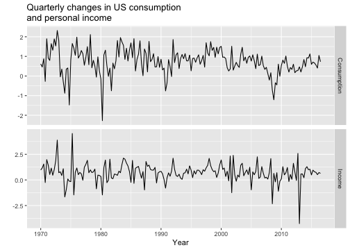
plot ηtηt and ϵtϵt
residuals function can be used to extract ηtηt and ϵtϵt.
library(magrittr)cbind("Regression Errors" = residuals(fit, type="regression"),"ARIMA errors" = residuals(fit, type="innovation")) %>%autoplot(facets=TRUE)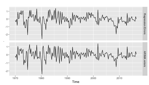
It is the ARIMA errors that should resemble a white noise series.
checkresiduals(fit)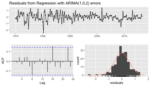
Ljung-Box testdata: Residuals from Regression with ARIMA(1,0,2) errorsQ* = 5.8916, df = 3, p-value = 0.117Model df: 5. Total lags used: 8Calculate forecasts
- We first need to forecast predictors
fcast <- forecast(fit, xreg=rep(mean(uschange[,2]),8))autoplot(fcast) + xlab("Year") + ylab("Percentage change")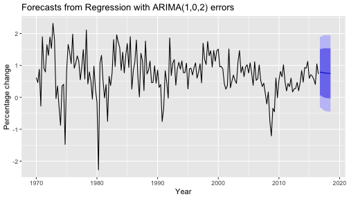
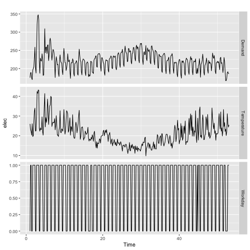
Forecasting electricity demand
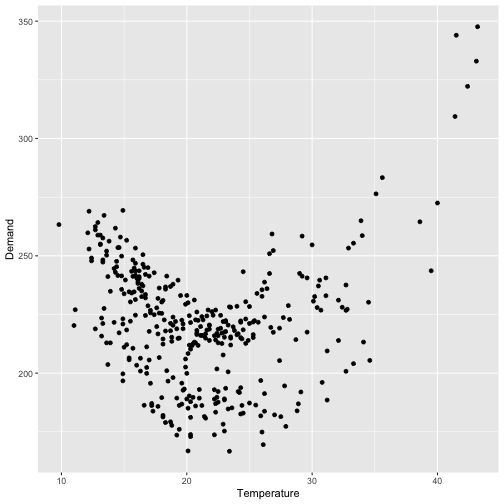
Model daily electricity demand as a function of temperature using quadratic regression with ARMA errors.
Forecasting electricity demand
Forecasting electricity demand (cont.)
checkresiduals(fit)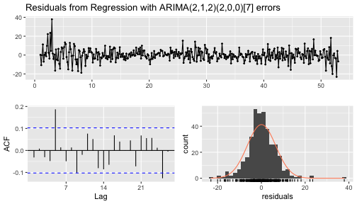
Ljung-Box testdata: Residuals from Regression with ARIMA(2,1,2)(2,0,0)[7] errorsQ* = 28.229, df = 4, p-value = 1.121e-05Model df: 10. Total lags used: 14autoplot(insurance, facets=TRUE) +xlab("Year") + ylab("") +ggtitle("Insurance advertising and quotations")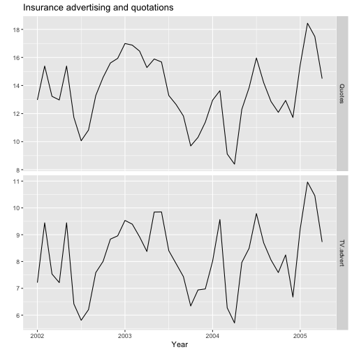
Generate forecasts
fc8 <- forecast(fit, h=20,xreg=cbind(AdLag0 = rep(8,20),AdLag1 = c(Advert[40,1], rep(8,19))))autoplot(fc8) + ylab("Quotes") +ggtitle("Forecast quotes with future advertising set to 8")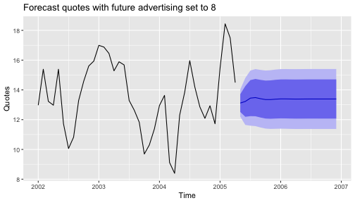
checkresiduals(fc8)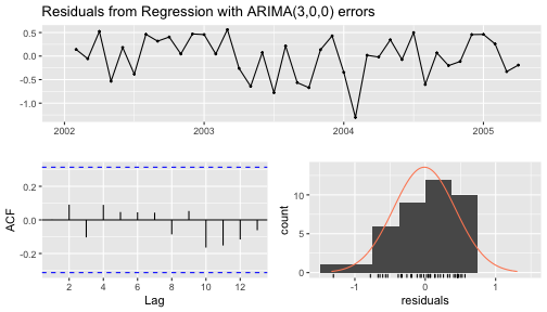
Ljung-Box testdata: Residuals from Regression with ARIMA(3,0,0) errorsQ* = 2.0324, df = 3, p-value = 0.5657Model df: 6. Total lags used: 9